Working with OpenTelemetry Traces

neard is instrumented in a few different ways. From the code perspective we have two major ways of instrumenting code:

• Prometheus metrics – by computing various metrics in code and expoding them via the prometheus crate.
• Execution tracing – this shows up in the code as invocations of functionality provided by the tracing crate.

The focus of this document is to provide information on how to effectively work with the data collected by the execution tracing approach to instrumentation.

Gathering and Viewing the Traces

Tracing the execution of the code produces two distinct types of data: spans and events. These then are exposed as either logs (representing mostly the events) seen in the standard output of the neard process or sent onwards to an opentelemetry collector.

When deciding how to instrument a specific part of the code, consider the following decision tree:

1. Do I need execution timing information? If so, use a span; otherwise
2. Do I need call stack information? If so, use a span; otherwise
3. Do I need to preserve information about inputs or outputs to a specific section of the code? If so, use key-values on a pre-existing span or an event; otherwise
4. Use an event if it represents information applicable to a single point of execution trace.

As of writing (February 2024) our codebase uses spans somewhat sparsely and relies on events heavily to expose information about the execution of the code. This is largely a historical accident due to the fact that for a long time stdout logs were the only reasonable way to extract information out of the running executable.

Today we have more tools available to us. In production environments and environments replicating said environment (i.e. GCP environments such as mocknet) there's the ability to push this data to Grafana Loki (for events) and Tempo (for spans and events alike), so long as the amount of data is within reason. For that reason it is critical that the event and span levels are chosen appropriately and in consideration with the frequency of invocations. In local environments developers can use projects like Jaeger, or set up the Grafana stack if they wish to use a consistent interfaces.

It is still more straightforward to skip all the setup necessary for tracing, but relying exclusively on logs only increases noise for the other developers and makes it ever so slightly harder to extract signal in the future. Keep this trade off in mind.

Spans

We have a style guide section on the use of Spans, please make yourself familiar with it.

Every tracing::debug_span!() creates a new span, and usually it is attached to its parent automatically.

However, a few corner cases exist.

• do_apply_chunks() starts 4 sub-tasks in parallel and waits for their completion. To make it work, the parent span is passed explicitly to the sub-tasks.

• Messages to actix workers. If you do nothing, that the traces are limited to work done in a single actor. But that is very restrictive and not useful enough. To workaround that, each actix message gets attached opentelemetry::Context. That context somehow represents the information about the parent span. This mechanism is the reason you see annoying .with_span_context() function calls whenever you send a message to an actix Actor.

• Inter-process tracing is theoretically available, but I have never tested it. The plan was to test it as soon as the Canary images get updated 😭 Therefore it most likely doesn’t work. Each PeerMessage is injected with TraceContext (1, 2) and the receiving node extracts that context and all spans generated in handling that message should be parented to the trace from another node.

• Some spans are created using info_span!() but they are few and mostly for the logs. Exporting only info-level spans doesn’t give any useful tracing information in Grafana.

• actix::Actor::handle() deserves a special note. The design choice was to provide a macro that lets us easily annotate every implementation of actix::Actor::handle(). This macro sets the following span attributes:

  • actor to the name of the struct that implements actix::Actor
  • handler to the name of the message struct

  And it lets you provide more span attributes. In the example, ClientActor specifies msg_type, which in all cases is identical to handler.

Configuration

The Tracing documentation page in nearone's Outline documents the steps necessary to start moving the trace data from the node to Nearone's Grafana Cloud instance. Once you set up your nodes, you can use the explore page to verify that the traces are coming through.

If the traces are not coming through quite yet, consider using the ability to set logging configuration at runtime. Create $NEARD_HOME/log_config.json file with the following contents:

{ "opentelemetry": "info" }

Or optionally with rust_log setting to reduce logging on stdout:

{ "opentelemetry": "info", "rust_log": "WARN" }

and invoke sudo pkill -HUP neard. Double check that the collector is running as well.

Good to know: You can modify the event/span/log targets you’re interested in just like when setting the RUST_LOG environment variable, including target filters. If you're setting verbose levels, consider selecting specific targets you're interested in too. This will help to keep trace ingest costs down.

For more information about the dynamic settings refer to core/dyn-configs code in the repository.

Local development

TODO: the setup is going to depend on whether one would like to use grafana stack or just jaeger or something else. We shoud document setting either of these up, including the otel collector and such for a full end-to-end setup. Success criteria: running integration tests should allow you to see the traces in your grafana/jaeger. This may require code changes as well.

Using the Grafana Stack here gives the benefit of all of the visualizations that are built-in. Any dashboards you build are also portable between the local environment and the Grafana Cloud instance. Jaeger may give a nicer interactive exploration ability. You can also set up both if you wish.

Visualization

Now that the data is arriving into the databases, it is time to visualize the data to determine what you want to know about the node. The only general advise I have here is to check that the data source is indeed tempo or loki.

Explore

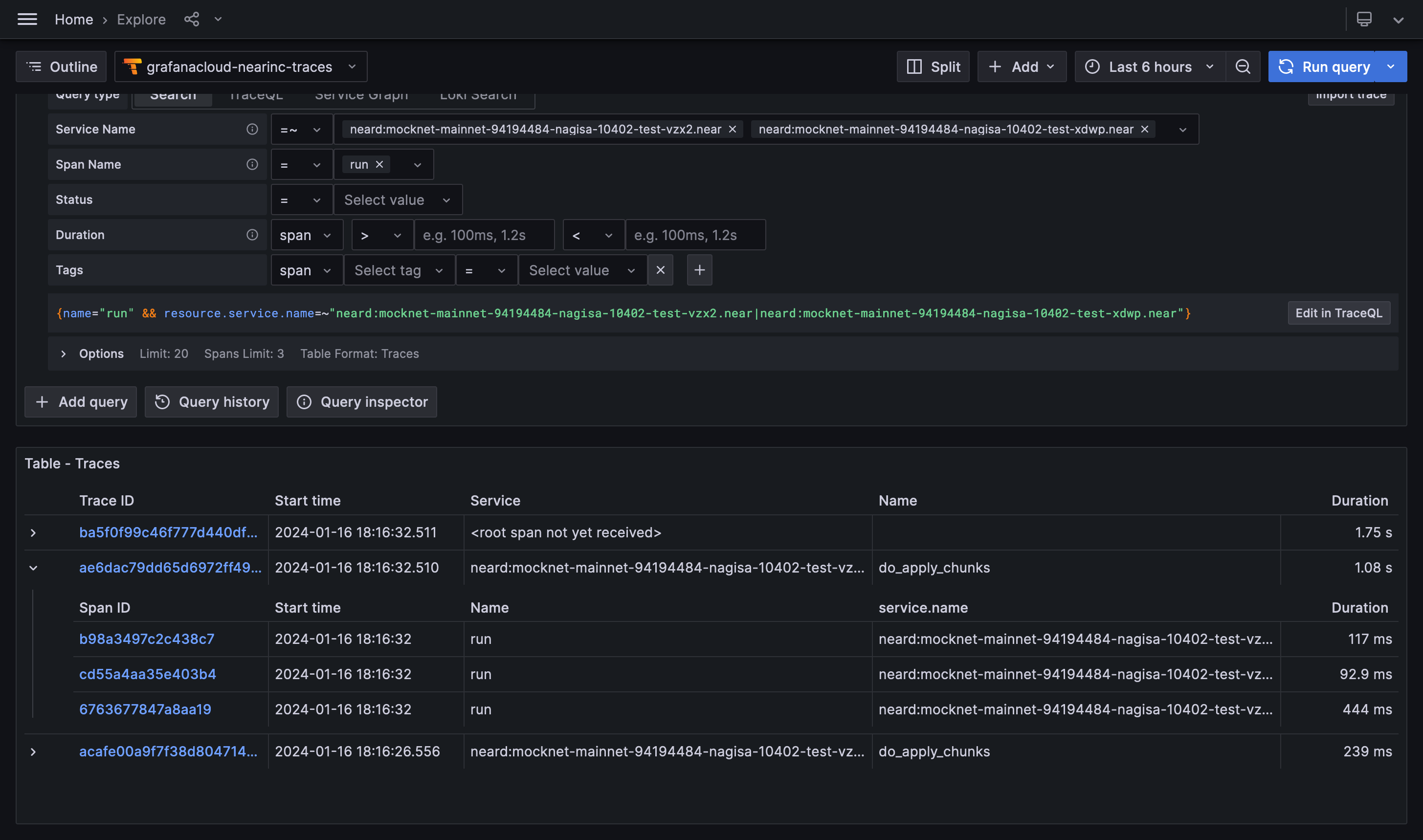
Initial exploration is best done with Grafana's Explore tool or some other mechanism to query and display individual traces.

The query builder available in Grafana makes the process quite straightforward to start with, but is also somewhat limited. Underlying TraceQL has many more features that are not available through the builder. For example, you can query data in somewhat of a relational manner, such as this query below queries only spans named process_receipt that take 50ms when run as part of new_chunk processing for shard 3!

{ name="new_chunk" && span.shard_id = "3" } >> { name="process_receipt" && duration > 50ms }

Good to know: When querying, keep in mind the "Options" dropdown that allows you to specify the limit of results and the format in which these results are presented! In particular, the "Traces/Spans" toggle will affect the durations shown in the result table.

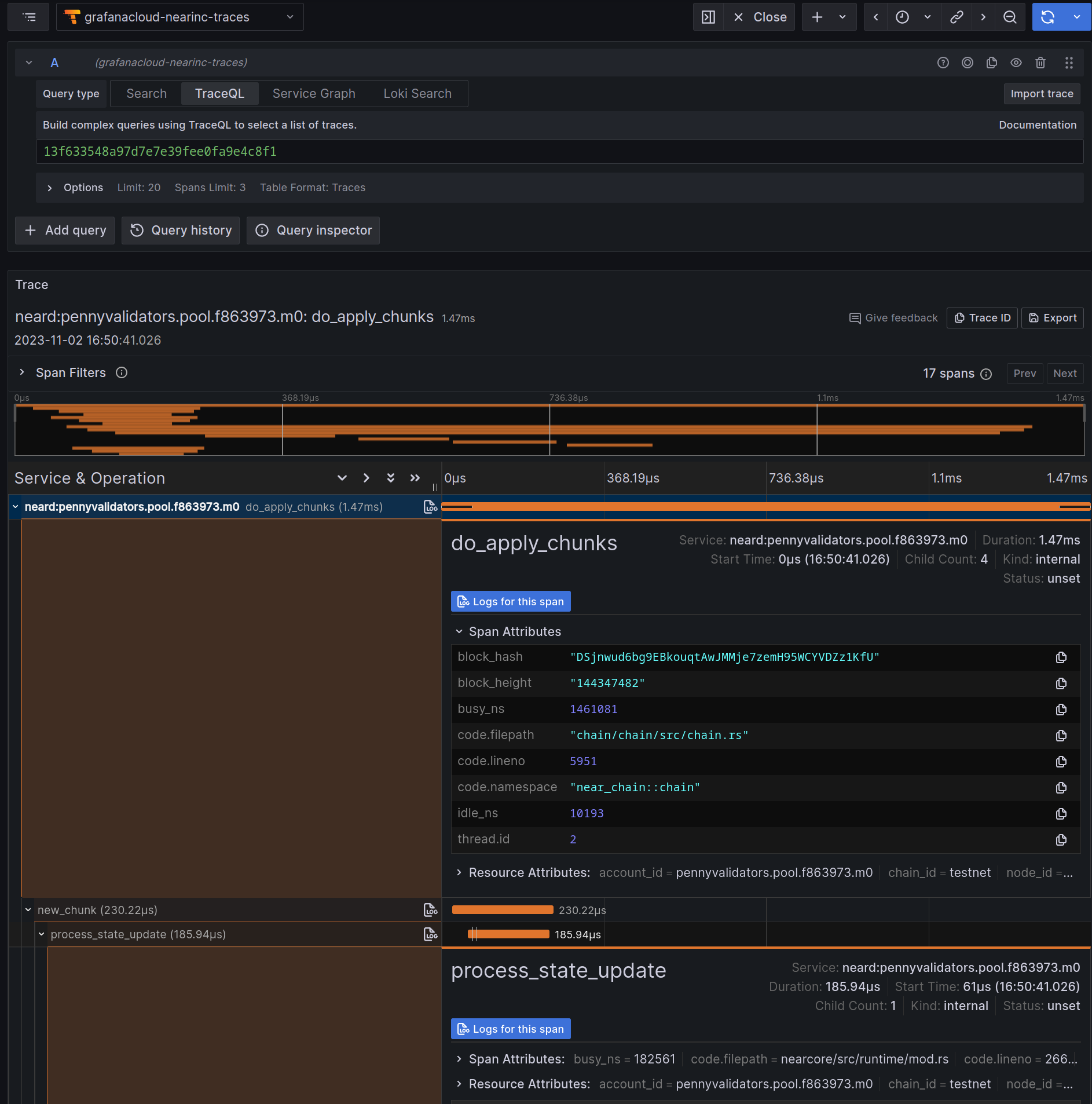
Once you click on a span of interest, Grafana will open you a view with the trace that contains said span, where you can inspect both the overall trace and the properties of the span:

Dashboards

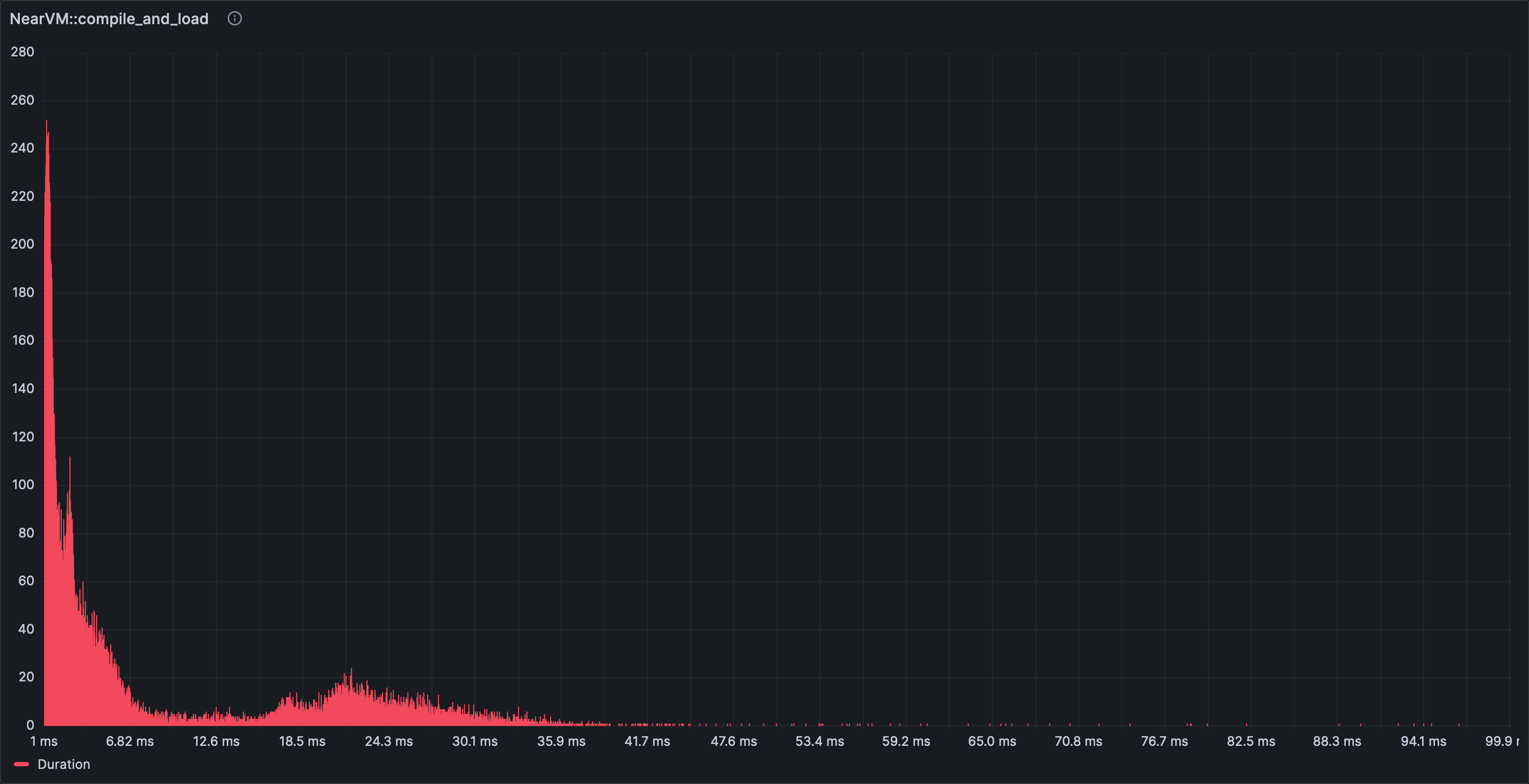
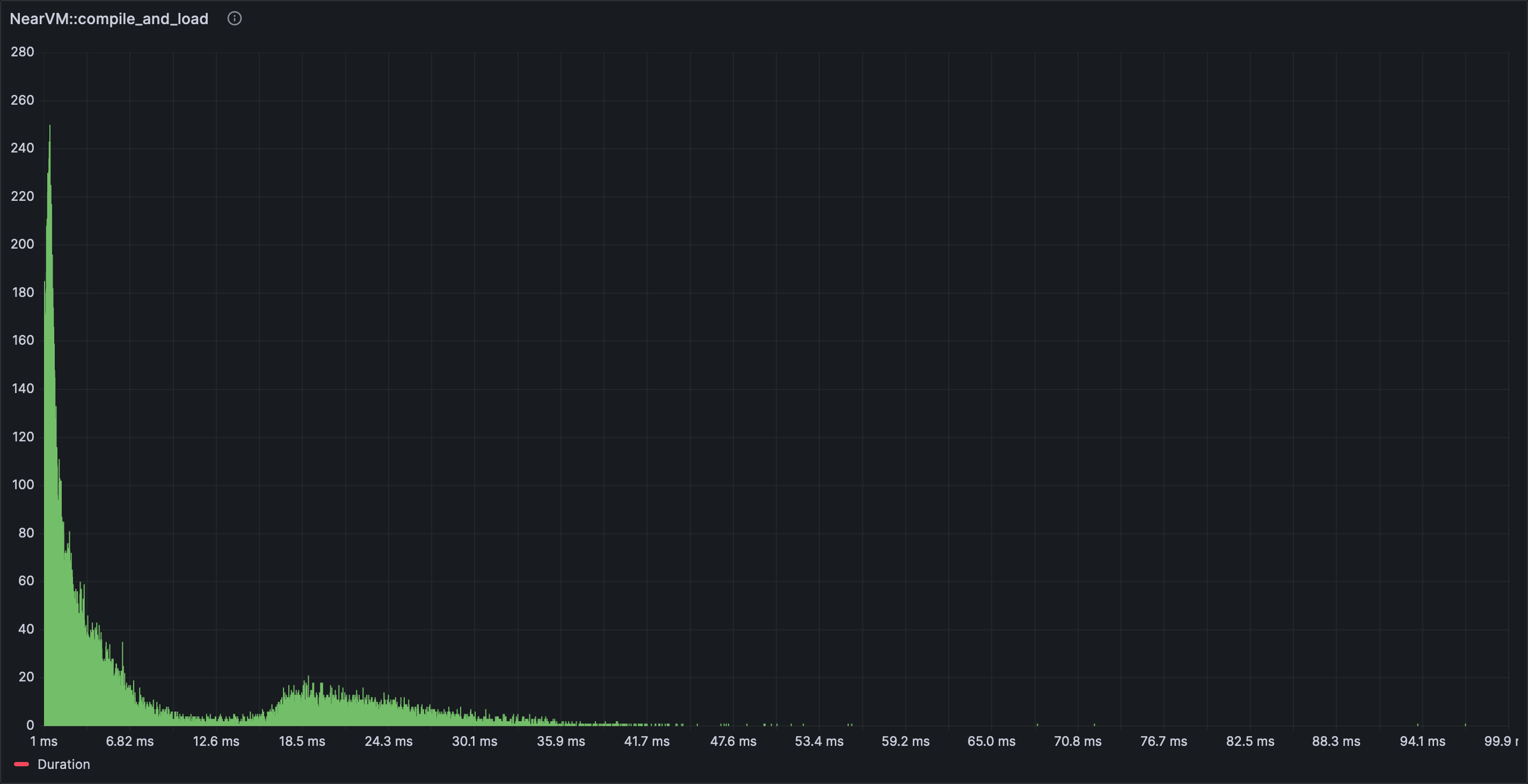
Once you have arrived at an interesting query, you may be inclined to create a dashboard that summarizes the data without having to dig into individual traces and spans.

As an example the author was interested in checking the execution speed before and after a change in a component. To make the comparison visual, the span of interest was graphed using the histogram visualization in order to obtain the following result. In this graph the Y axis displays the number of occurrences for spans that took X-axis long to complete.

In general most of the panels work with tracing results directly but some of the most interesting ones do not. It is necessary to experiment with certain options and settings to have grafana panels start showing data. Some notable examples:

1. Time series – a “Prepare time series” data transformation with “Multi-frame time series” has to be added;
2. Histogram – make sure to use "spans" table format option;
3. Heatmap - set “Calculate from data” option to “Yes”;
4. Bar chart – works out of the box, but x axis won't be readable ever.

You can also add a panel that shows all the trace events in a log-like representation using the log or table visualization.

Multiple nodes

One frequently asked question is whether Grafana lets you distinguish between nodes that export tracing information.

The answer is yes.

In addition to span attributes, each span has resource attributes. There you'll find properties like node_id which uniquely identify a node.

• account_id is the account_id from validator_key.json;
• chain_id is taken from genesis.json;
• node_id is the public key from node_key.json;
• service.name is account_id if that is available, otherwise it is node_id.